3 Smart Ways to Encode Categorical Features for Machine Learning
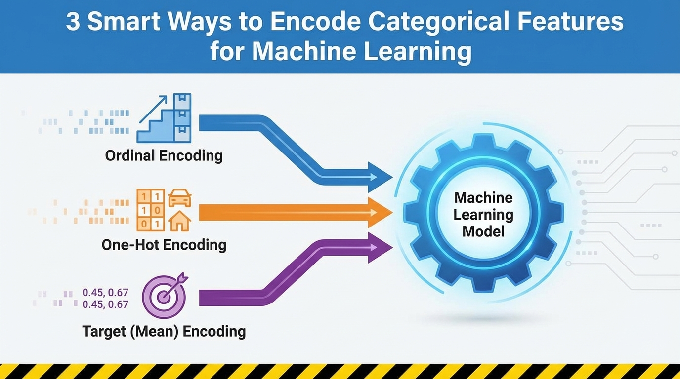
In this article, you will learn three reliable techniques — ordinal encoding, one-hot encoding, and target (mean) encoding — for turning categorical features into model-ready numbers while preserving their meaning.
Topics we will cover include:
- When and how to apply ordinal (label-style) encoding for truly ordered categories.
- Using one-hot encoding safely for nominal features and understanding its trade-offs.
- Applying target (mean) encoding for high-cardinality features without leaking the target.
Time to get to work.

3 Smart Ways to Encode Categorical Features for Machine Learning
Image by Editor
Introduction
If you spend any time working with real-world data, you quickly realize that not everything comes in neat, clean numbers. In fact, most of the interesting aspects, the things that define people, places, and products, are captured by categories. Think about a typical customer dataset: you’ve got fields like City, Product Type, Education Level, or even Favorite Color. These are all examples of categorical features, which are variables that can take on one of a limited, fixed number of values.
The problem? While our human brains seamlessly process the difference between “Red” and “Blue” or “New York” and “London,” the machine learning models we use to make predictions can’t. Models like linear regression, decision trees, or neural networks are fundamentally mathematical functions. They operate by multiplying, adding, and comparing numbers. They need to calculate distances, slopes, and probabilities. When you feed a model the word “Marketing,” it doesn’t see a job title; it just sees a string of text that has no numerical value it can use in its equations. This inability to process text is why your model will crash instantly if you try to train it on raw, non-numeric labels.
The primary goal of feature engineering, and specifically encoding, is to act as a translator. Our job is to convert these qualitative labels into quantitative, numerical features without losing the underlying meaning or relationships. If we do it right, the numbers we create will carry the predictive power of the original categories. For instance, encoding must ensure that the number representing a high-level Education Level is quantitatively “higher” than the number representing a lower level, or that the numbers representing different Cities reflect their difference in purchase habits.
To tackle this challenge, we have evolved smart ways to perform this translation. We’ll start with the most intuitive methods, where we simply assign numbers based on rank or create separate binary flags for each category. Then, we’ll move on to a powerful technique that uses the target variable itself to build a single, dense feature that captures a category’s true predictive influence. By understanding this progression, you’ll be equipped to choose the perfect encoding method for any categorical data you encounter.
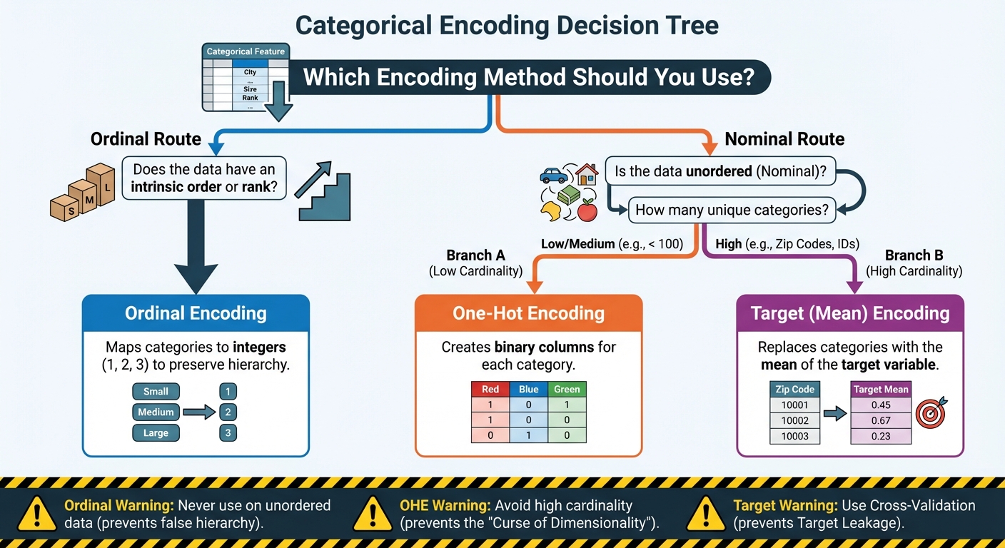
3 Smart Ways to Encode Categorical Features for Machine Learning: A Flowchart (click to enlarge)
Image by Editor
1. Preserving Order: Ordinal and Label Encoding
The first, and simplest, translation technique is designed for categorical data that isn’t just a collection of random names, but a set of labels with an intrinsic rank or order. This is the key insight. Not all categories are equal; some are inherently “higher” or “more” than others.
The most common examples are features that represent some sort of scale or hierarchy:
- Education Level: (High School => College => Master’s => PhD)
- Customer Satisfaction: (Very Poor => Poor => Neutral => Good => Excellent)
- T-shirt Size: (Small => Medium => Large)
When you encounter data like this, the most effective way to encode it is to use Ordinal Encoding (often informally called “label encoding” when mapping categories to integers).
The Mechanism
The process is straightforward: you map the categories to integers based on their position in the hierarchy. You don’t just assign numbers randomly; you explicitly define the order.
For example, if you have T-shirt sizes, the mapping would look like this:
| Original Category | Assigned Numerical Value |
|---|---|
| Small (S) | 1 |
| Medium (M) | 2 |
| Large (L) | 3 |
| Extra-Large (XL) | 4 |
By doing this, you are teaching the machine that an XL (4) is numerically “more” than an S (1), which correctly reflects the real-world relationship. The difference between an M (2) and an L (3) is mathematically the same as the difference between an L (3) and an XL (4), a unit increase in size. This resulting single column of numbers is what you feed into your model.
Introducing a False Hierarchy
While Ordinal Encoding is the perfect choice for ordered data, it carries a major risk when misapplied. You must never use it on nominal (non-ordered) data.
Consider encoding a list of colors: Red, Blue, Green. If you arbitrarily assign them: Red = 1, Blue = 2, Green = 3, your machine learning model will interpret this as a hierarchy. It will conclude that “Green” is twice as large or important as “Red,” and that the difference between “Blue” and “Green” is the same as the difference between “Red” and “Blue.” This is almost certainly false and will severely mislead your model, forcing it to learn non-existent numerical relationships.
The rule here is simple and firm: use Ordinal Encoding only when there is a clear, defensible rank or sequence between the categories. If the categories are just names without any intrinsic order (like types of fruit or cities), you must use a different encoding technique.
Implementation and Code Explanation
We can implement this using the OrdinalEncoder from scikit-learn. The key is that we must explicitly define the order of the categories ourselves.
|
1 2 3 4 5 6 7 8 9 10 11 12 13 14 15 16 17 18 19 20 |
from sklearn.preprocessing import OrdinalEncoder import numpy as np
# Sample data representing customer education levels data = np.array([[‘High School’], [‘Bachelor\’s’], [‘Master\’s’], [‘Bachelor\’s’], [‘PhD’]])
# Define the explicit order for the encoder # This ensures that ‘Bachelor\’s’ is correctly ranked below ‘Master\’s’ education_order = [ [‘High School’, ‘Bachelor\’s’, ‘Master\’s’, ‘PhD’] ]
# Initialize the encoder and pass the defined order encoder = OrdinalEncoder(categories=education_order)
# Fit and transform the data encoded_data = encoder.fit_transform(data)
print(“Original Data:\n”, data.flatten()) print(“\nEncoded Data:\n”, encoded_data.flatten()) |
In the code above, the critical part is setting the categories parameter when initializing OrdinalEncoder. By passing the exact list education_order, we tell the encoder that ‘High School’ comes first, then ‘Bachelor’s’, and so on. The encoder then assigns the corresponding integers (0, 1, 2, 3) based on this custom sequence. If we had skipped this step, the encoder might have assigned the integers based on alphabetical order, which would destroy the meaningful hierarchy we wanted to preserve.
2. Eliminating Rank: One-Hot Encoding (OHE)
As we discussed, Ordinal Encoding only works if your categories have a clear rank. But what about features that are purely nominal, meaning they have names, but no inherent order? Think about things like Country, Favorite Animal, or Gender. Is “France” better than “Japan”? Is “Dog” mathematically greater than “Cat”? Absolutely not.
For these non-ordered features, we need a way to encode them numerically without introducing a false sense of hierarchy. The solution is One-Hot Encoding (OHE), which is by far the most widely used and safest encoding technique for nominal data.
The Mechanism
The core idea behind OHE is simple: instead of replacing a single category column with a single number, it is replaced with multiple binary columns. For every unique category in your original feature, you create a brand-new column. These new columns are often called dummy variables.
For example, if your original Color feature has three unique categories (Red, Blue, Green), OHE will create three new columns: Color_Red, Color_Blue, and Color_Green.
In any given row, only one of those columns will be “hot” (a value of 1), and the rest will be 0.
| Original Color | Color_Red | Color_Blue | Color_Green |
|---|---|---|---|
| Red | 1 | 0 | 0 |
| Blue | 0 | 1 | 0 |
| Green | 0 | 0 | 1 |
This method is brilliant because it completely solves the hierarchy problem. The model now treats each category as a completely separate, independent feature. “Blue” is no longer numerically related to “Red”; it just exists in its own binary column. This is the safest and most reliable default choice when you know your categories have no order.
The Trade-off
While OHE is the standard for features with low to medium cardinality (i.e., a small to moderate number of unique values, typically under 100), it quickly becomes a problem when dealing with high-cardinality features.
Cardinality refers to the number of unique categories in a feature. Consider a feature like Zip Code in the United States, which could easily have over 40,000 unique values. Applying OHE would force you to create 40,000 brand-new binary columns. This leads to two major issues:
- Dimensionality: You suddenly balloon the width of your dataset, creating a massive, sparse matrix (a matrix containing mostly zeros). This dramatically slows down the training process for most algorithms.
- Overfitting: Many categories will only appear once or twice in your dataset. The model might assign an extreme weight to one of these rare, specific columns, essentially memorizing its one appearance rather than learning a general pattern.
When a feature has thousands of unique categories, OHE is simply impractical. This limitation forces us to look beyond OHE and leads us directly to our third, more advanced technique for dealing with data at a massive scale.
Implementation and Code Explanation
In Python, the OneHotEncoder from scikit-learn or the get_dummies() function from pandas are the standard tools. The pandas method is generally easier for quick transformation:
|
import pandas as pd
# Sample data with a nominal feature: Color data = pd.DataFrame({ ‘ID’: [1, 2, 3, 4, 5], ‘Color’: [‘Red’, ‘Blue’, ‘Red’, ‘Green’, ‘Blue’] })
# 1. Apply One-Hot Encoding using pandas get_dummies df_encoded = pd.get_dummies(data, columns=[‘Color’], prefix=‘Is’)
print(df_encoded) |
In this code, we pass our DataFrame data and specify the column we want to transform (Color). The prefix='Is' simply adds a clean prefix (like ‘Is_Red‘) to the new columns for better readability. The output DataFrame retains the ID column and replaces the single Color column with three new, independent binary features: Is_Red, Is_Blue, and Is_Green. A row that was originally ‘Red’ now has a 1 in the Is_Red column and a 0 in the others, achieving the desired numerical separation without imposing rank.
3. Harnessing Predictive Power: Target (Mean) Encoding
As we established, One-Hot Encoding fails spectacularly when a feature has high cardinality, thousands of unique values like Product ID, Zip Code, or Email Domain. Creating thousands of sparse columns is computationally inefficient and leads to overfitting. We need a technique that can compress these thousands of categories into a single, dense column without losing their predictive signal.
The answer lies in Target Encoding, also frequently called Mean Encoding. Instead of relying only on the feature itself, this method strategically uses the target variable (Y) to determine the numerical value of each category.
The Concept and Mechanism
The core idea is to encode each category with the average value of the target variable for all data points belonging to that category.
For instance, imagine you are trying to predict if a transaction is fraudulent (Y=1 for fraud, Y=0 for legitimate). If your categorical feature is City:
- You group all transactions by City
- For each city, you calculate the mean of the Y variable (the average fraud rate)
- The city of “Miami” might have an average fraud rate of 0.10 (or 10%), and “Boston” might have 0.02 (2%)
- You replace the categorical label “Miami” in every row with the number 0.10, and “Boston” with 0.02
The result is a single, dense numerical column that immediately embeds the predictive power of that category. The model instantly knows that rows encoded with 0.10 are ten times more likely to be fraudulent than rows encoded with 0.01. This drastically reduces dimensionality while maximizing information density.
The Advantage and The Critical Danger
The advantage of Target Encoding is clear: it solves the high-cardinality problem by replacing thousands of sparse columns with just one dense, powerful feature.
However, this method is often called “the most dangerous encoding technique” because it is extremely vulnerable to Target Leakage.
Target leakage occurs when you inadvertently include information in your training data that would not be available at prediction time, leading to artificially perfect (and useless) model performance.
The Fatal Mistake: If you calculate the average fraud rate for Miami using all the data, including the row you are currently encoding, you are leaking the answer. The model learns a perfect correlation between the encoded feature and the target variable, essentially memorizing the training data instead of learning generalizable patterns. When deployed on new, unseen data, the model will fail spectacularly.
Preventing Leakage
To use Target Encoding safely, you must ensure that the target value for the row being encoded is never used in the calculation of its feature value. This requires advanced techniques:
- Cross-Validation (K-Fold): The most robust approach is to use a cross-validation scheme. You split your data into K folds. When encoding one fold (the “holdout set”), you calculate the target mean only using the data from the other K-1 folds (the “training set”). This ensures the feature is generated from out-of-fold data.
- Smoothing: For categories with very few data points, the calculated mean can be unstable. Smoothing is applied to “shrink” the mean of rare categories toward the global average of the target variable, making the feature more robust. A common smoothing formula often involves weighting the category mean with the global mean based on the sample size.
Implementation and Code Explanation
Implementing safe Target Encoding usually requires custom functions or advanced libraries like category_encoders, as scikit-learn’s core tools don’t offer built-in leakage protection. The key principle is calculating the means outside of the primary data being encoded.
For demonstration, we’ll use a conceptual example, focusing on the result of the calculation:
|
1 2 3 4 5 6 7 8 9 10 11 12 13 14 15 16 17 18 19 20 21 22 23 24 |
import pandas as pd
# Sample data data = pd.DataFrame({ ‘City’: [‘Miami’, ‘Boston’, ‘Miami’, ‘Boston’, ‘Boston’, ‘Miami’], # Target (Y): 1 = Fraud, 0 = Legitimate ‘Fraud_Target’: [1, 0, 1, 0, 0, 0] })
# 1. Calculate the raw mean (for demonstration only — this is UNSAFE leakage) # Real-world use requires out-of-fold means for safety! mean_encoding = data.groupby(‘City’)[‘Fraud_Target’].mean().reset_index() mean_encoding.columns = [‘City’, ‘City_Encoded_Value’]
# 2. Merge the encoded values back into the original data df_encoded = data.merge(mean_encoding, on=‘City’, how=‘left’)
# Output the calculated means for illustration miami_mean = df_encoded[df_encoded[‘City’] == ‘Miami’][‘City_Encoded_Value’].iloc[0] boston_mean = df_encoded[df_encoded[‘City’] == ‘Boston’][‘City_Encoded_Value’].iloc[0]
print(f“Miami Encoded Value: {miami_mean:.4f}”) print(f“Boston Encoded Value: {boston_mean:.4f}”) print(“\nFinal Encoded Data (Conceptual Leakage Example):\n”, df_encoded) |
In this conceptual example, “Miami” has three records with target values [1, 1, 0], giving an average (mean) of 0.6667. “Boston” has three records [0, 0, 0], giving an average of 0.0000. The raw city names are replaced by these float values, dramatically increasing the feature’s predictive power. Again, to use this in a real project, the City_Encoded_Value would need to be calculated carefully using only the subset of data not being trained on, which is where the complexity lies.
Conclusion
We’ve covered the journey of transforming raw, abstract categories into the numerical language that machine learning models demand. The difference between a model that works and one that excels often comes down to this feature engineering step.
The key takeaway is that no single technique is universally superior. Instead, the right choice depends entirely on the nature of your data and the number of unique categories you are dealing with.
To quickly summarize the three smart approaches we’ve detailed:
- Ordinal Encoding: This is your solution when you have an intrinsic rank or hierarchy among your categories. It is efficient, adding only one column to your dataset, but it must be reserved exclusively for ordered data (like sizes or levels of agreement) to avoid introducing misleading numerical relationships.
- One-Hot Encoding (OHE): This is the safest default when dealing with nominal data where order doesn’t matter and the number of categories is small to medium. It prevents the introduction of false rank, but you must be wary of using it on features with thousands of unique values, as it can balloon the dataset size and slow down training.
- Target (Mean) Encoding: This is the powerful answer for high-cardinality features that would overwhelm OHE. By encoding the category with its mean relationship to the target variable, you create a single, dense, and highly predictive feature. However, because it uses the target variable, it demands extreme caution and must be implemented using cross-validation or smoothing to prevent catastrophic target leakage.